Natural gas’ volatility stems from a unique supply-demand balance. On the one hand, demand is highly inelastic. In winter, gas is used to heat homes, offices, factories and so on. The colder it is, the more gas is burned for space heating purposes. People don’t stop heating their homes altogether because prices are high. On the other hand, supply is (in the short-term) relatively fixed.ⁱ Production is not “controllable” because gas wells produce gas at a rate determined by geological and technological factors.

In effect, during winter, demand is an unstoppable force while supply is an immovable object. When the two meet, prices spike.

On the other hand, during periods of relatively low consumption such as spring, summer and fall, the inelasticity of demand returns to haunt the gas market. People are not going to heat their homes if the weather is moderate or hot. But production remains relatively fixed. Now, supply is an unstoppable force while demand is an immovable object. When the two meet, prices drop.

The chart below vividly illustrates the seasonality and inelasticity of demand as well as the fixed nature of supply. Notice how demand (red) dramatically exceeds supply (black) during winters.

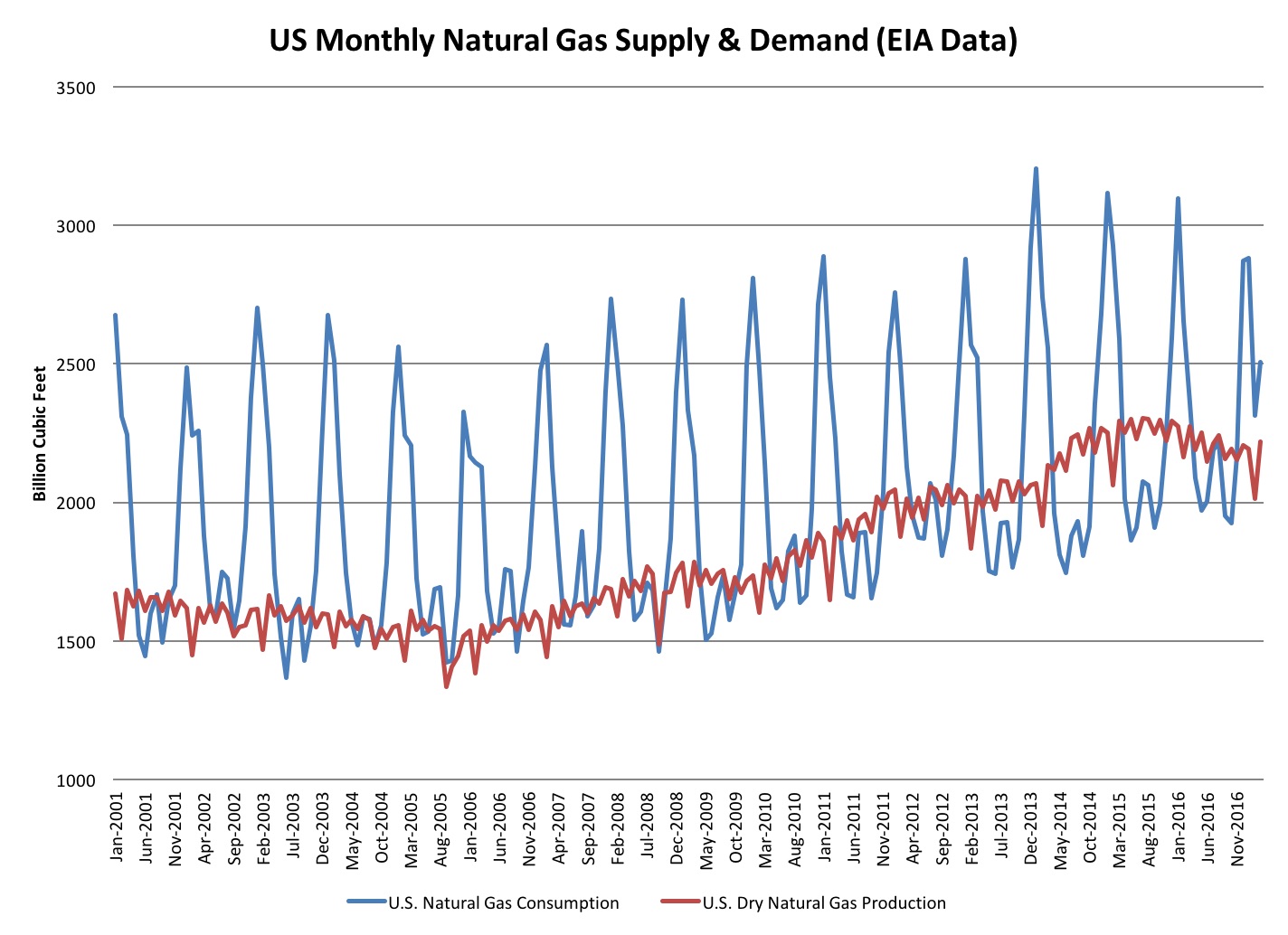
Therefore, the only way to bridge the enormous gap between supply and demand during winter is storage. During periods of relatively low consumption, such as the seven months from April through October, excess supply can be injected into storage. During periods of elevated consumption, such as the five months from November through March, gas is withdrawn from storage to meet demand. Thus, storage is a time arbitrage – buy today to sell a certain number of months from now.

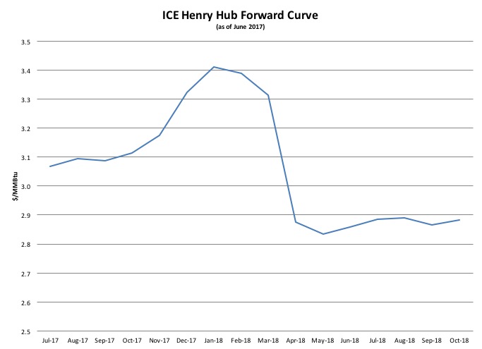
This structural imbalance is reflected in gas market prices. Specifically, for any given 12 month period, futures prices for the April-October strip are lower than futures prices for the November-March strip (see chart below). Looking at individual months, January and February futures are the highest prices of the year while April and May are typically the lowest prices of the year. At the time of writing, the price difference between October futures and January futures is 12% (ICE futures settlements as of 2-18-2015).

In theory, the price differential between slack months and peak months should be driven primarily by the cost of storage. The reality is more complex.

During winter, demand is the key to the price of gas. Since heating demand is highly inelastic, the only way to materially reduce demand is to reduce consumption by gas-fired power plants. Without going into the technical details of how that is accomplished, suffice it to say that natural gas typically has to become more expensive than heating oil or residual fuel to trigger a material drop in demand from gas-fired power plants.

During summer, the dynamic is more complex. Since storage users can inject gas into storage at today’s price for delivery in, say, January, they need a powerful incentive to sell gas into the spot market. Thus, during heat waves, the spot market price has to increase to the point where it exceeds enough storage users’ utility function of the time value of money to get them to sell. As if this wasn’t complex enough, weather forecasting being what it is, the market has no way of knowing how high demand will be next month – let alone next winter. Therefore, it has to continuously monitor the current supply-demand balance to estimate whether enough gas will be injected into storage by the end of October to meet winter demand or withdrawn from storage by the end of April to meet storage restrictions. This can cause significant intramonth price fluctuations.

Storage operators require stored gas to be at or below certain levels in the March-April period. This ensures there is enough room to accommodate injections during the next April-October cycle. In an extreme situation, any gas above those levels is subject to “ratchets” or injection limitations; excess gas cannot be injected and is therefore dumped onto the spot market at whatever price the market will pay.

If there is a lot of gas left in storage, ratchets can precipitate a price collapse in the spot market for gas in spring. The spot market for gas is called the “cash market” and consists primarily of trades for physical gas delivered the next business day or the next weekend strip (Saturday, Sunday and Monday). If gas is being dumped out of storage at the same time as producers are attempting to bring current production to market, there is a swift race to the bottom. In 2012, cash prices dropped as low as $1.82/MMBtu in April before rebounding to $3.50/MMBtu by November (EIA Henry Hub Spot Gas prices). Injecting that spring and withdrawing that winter was a classic storage time arbitrage - one undertaken at some risk, of course. To the extent the market is pricing in the probability of ratchets creating distressed gas, March and April futures contracts may start to fall as early as December.

At the other end of the time scale, storage facilities can only accommodate a certain amount of gas. As the April-October filling season goes on, storage operators manage the rate at which gas can be injected into storage to avoid a “garage full” scenario. If storage levels are high, they may begin to restrict which categories of users can inject gas in what quantities. If production has increased materially and/or the summer has been unusually mild (reducing air-conditioning demand and, therefore, demand for gas from gas-fired power plants), storage restrictions could force another race to the bottom in the fall as producers compete to sell gas into the cash market.

Putting it all together, storage is critical to the way the market functions and to price formation. It is, as mentioned, a time arbitrage. It also has significant embedded optionality. Depending on how flexible the storage facility is and how many times the user can inject/withdraw from storage, multiple strategies can be used to monetize this embedded optionality. A few popular examples:

• Fully Hedged Seasonal: Inject during the April-October period and sell during the November-March period. Hedge both sides by buying (andtaking delivery of) the April-October futures strip and selling (and making delivery of) theNovember-March futures strip
• Partially Hedged Seasonal: Inject by buying opportunistically in the cash market during the April-October period and selling (and makingdelivery of) the November-March futures strip
• Distressed Gas: Buy gas in the cash market when ”garage full” scenarios seem to be more likely and sell months later when the market resets (or sell futures today to lock in gains)
• Cash-futures spreads: Cash market prices can delink from futures prices because futures may be anticipating a different supply-demand balance a few weeks/months into the future than the one that exists today. By buying today and selling the futures, you capture the spread between the two and help make the overall market more efficient

Other, more complex strategies exist but they are beyond the scope of this paper.

There are risks involved in storage, too.

• The cost and flexibility of the storage determines the range of strategies and associated risk/reward available to the user
• Collateral and credit requirements can be stringent, with attendant cash flow implications. Injecting into storage can require paying in full for the gas injected (100% collateralization) while a futures sale into a rising market requires the user to post more margin until the trade is unwound
• Changes in market conditions can make the injected gas worth significantly less than what the user paid
• Time value of money utility functions need to be defined. Put another way, there is potentially a very high opportunity cost to injecting into/withdrawing from storage today instead of next week

Owing to the physical nature of the storage business and the complexities involved, only some of which have been discussed here, storage has typically been limited to physical operators, merchant commodity firms, utilities and large end-users, banks with physical trading platforms and so on. However, thanks to the evolution of the futures and options markets there are ways to participate in the time arbitrage phenomenon.

Time spreads (or calendar spreads) are a popular way to participate in these markets alongside the storage operators. We have discussed the April-October and November-March strips. As more data becomes available, the price differential between those two strips may increase or decrease. At a more granular level, the October/November and October/January futures spreads have historically been two popular “filling season” spreads. The October/November spread is the price differential between the November future and the October future while the October/January spread is the price differential between the January future and the October future. As the filling season goes on, the storage-driven demand for spot gas fluctuates and the market begins to price in the probability of a “garage full” scenario. If injections have been high and the probability of a distressed gas situation is increasing, the October future will start to trade at a greater discount to November (when demand begins to pick up) and January (when winter demand has kicked in fully). The spread will widen when storage is ample and vice versa. The March/April spread has historically been a popular “withdrawal season” spread. If storage is low and there is a risk gas prices will have to approach heating oil prices, gas for delivery in March (when it is still cold and every molecule counts) could be far more valuable than gas for delivery in April – and the March future would be a significant premium to the April future. The spread will widen when storage is low and vice versa.

Since ICE has defined these spreads as discrete tradable products, the trader does not have to worry about pricing the individual legs and executing them efficiently. He/she can simply trade the predefined spread product and focus on his/her view of the spreads instead. These spread contracts are highly liquid and do not require physical gas infrastructure.

Another way of participating in time arbitrage is Calendar Spread Options, which are options written on the calendar spreads mentioned above. However, they are complex and volatile structures which are beyond the scope of this paper.

Time spreads do not provide the ultimate granularity and optionality that physical storage does because of the nature of futures contracts. Financially-settled futures contracts expire. The molecules injected into storage do not “disappear”. Since the natural gas forward curve is typically in contango for the April-February strip, the financial participant loses money each time the contract expires and he/she has to roll his position into the next month. The only way around that is to actively pick and choose when to roll the contract – which brings its own risks. The storage participant pays a flat fee and can ride the contango until he/she decides to sell the gas.

Additionally, the storage participant can choose to buy/sell gas intra-month in the cash market – something the financial trader cannot do. At times the cash-futures spread can be as high as 10%. Depending on the flexibility of their storage, storage participants can capture this differential several times over the course of a year.

There is a way to obtain that extra granularity and optionality. Using ICE financially-settled swing swap futures, a financial participant can transact gas at the cash market price for any given day or strip of days inside the month. In effect, the financial participant buys/sells financially-settled gas at close to the price physical storage participants are injecting/withdrawing gas from storage. Under circumstances which are beyond the scope of this paper and should be discussed with a sophisticated market advisor, it may be possible to use that ICE swing swap future functionality to create a virtual equivalent to physical storage and trade gas intramonth and inter-month in ways similar to those enjoyed by storage participants. However, this brings its own unique risks with it and requires the services of sophisticated counterparties and advisors.

Natural gas is one of the most volatile publicly traded commodities in the world due to its unique inventory constraints and supply-demand characteristics. For both physical storage participants and financial participants, this provides unique opportunities to manage risk and enhance returns. For the sophisticated financial participant, exchange products provide the building blocks for niche strategies that can sustainably generate true alpha.

ⁱWell freezes and hurricane-related shut-ins can affect supply in the short-term, but are outside the scope of this paper. We are focused on the big picture here.

This white paper has been prepared exclusively for Intercontinental Exchange Inc. (“ICE”) by Jaya S. Bajpai. This material has been prepared for informational purposes only. This material is not to be construed as a recommendation; or an offer to buy or sell; or the solicitation of an offer to buy or sell any security, financial product, or instrument; or to participate in any particular trading strategy. Certain transactions, including those involving futures, options, and high-yield securities, give rise to substantial risk and are not suitable for all investors. Independent advisors should be consulted. Jaya S. Bajpai, Seattle City Light and ICE do not make any recommendations regarding the merit of any company, security or other financial product or investment identified in this document, nor do they make any recommendation regarding the purchase or sale of any such company, security, financial product or investment that may be described or referred to in this document.

The information provided in this paper has been obtained from sources believed to be reliable, but is not guaranteed by ICE or its subsidiaries or by Seattle City Light, as to accuracy or completeness and is intended for purposes of information and education only.